Die neuen Import Formate sind ExpressionML, FITS, MathML, NB, NotebookML, SDTS, SymbolicXML, XML.
Die neuen Export Formate sind ExpressionML, FITS, MathML, NB, NotebookML, SVG, techexplorer, XML.
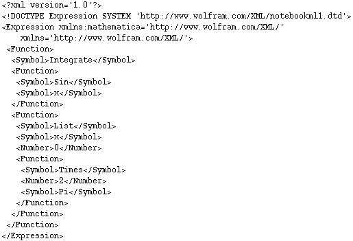
Notebooks und Ausdrücke können mit Hilfe der neuen XML Erweiterungen im Standard XML Format abgespeichert werden. Das folgende Beispiel zeigt wie man einen Mathematica Ausdruck in ExpressionML umwandelt.
![]()
![]()
Mathematica 4.2 unterstützt das Flexible Image Transport System (FITS) Format, ein logisches Datenformat entwickelt von Astronomen für den Austausch astronischer Daten. Der Standard wird von der International Astronomical Union kontrolliert. Das FITS Format wird bei der NASA als Standarddatenformat benutzt.
Die Option ConversionOptions kann benutzt werden um Header-Informationen mit zu importieren.
Beispieldateien im FITS Format sind auf http://www.cv.nrao.edu/fits/data/tests/incunabula/mssso82/ zu finden.
Mit Hilfe des J/Link GetURL Beispielprogramms kann eine beliebige Binärdatei vom Internet auf die Festplatte geladen werden.
Needs["JLink`"]
$ProxyHost=None;
$ProxyPort=8080;
Options[GetURL]={ProxyHost :> $ProxyHost,
ProxyPort :> $ProxyPort};
GetURL[url_String, opts___?OptionQ] :=
JavaBlock[
Module[{u, stream, numRead, outFile, buf, prxyHost, prxyPort},
{prxyHost, prxyPort} = {ProxyHost, ProxyPort} /. Flatten[{opts}] /. Options[GetURL];
StartJava[];
If[StringQ[prxyHost],
(* Set properties to force use of proxy. *)
SetInternetProxy[prxyHost, prxyPort]
];
u = JavaNew["java.net.URL", url];
(* This is where the error will show up if the URL is not valid.
A Java exception will be thrown during openStream, which
causes the method to return $Failed.
*)
stream = u@openStream[];
If[stream === $Failed, Return[$Failed]];
buf = JavaNew["[B", 5000]; (* 5000 is an arbitrary buffer size *)
outFile = OpenTemporary[DOSTextFormat->False];
While[(numRead = stream@read[buf]) > 0,
WriteString[outFile, FromCharacterCode[If[# < 0, # + 256, #]& /@ Take[Val[buf], numRead]]]
];
stream@close[];
Close[outFile] (* Close returns the filename *)
]
]
Mit Hilfe des J/Link GetURL Beispielprogramms http://www.cv.nrao.edu/fits/data/tests/incunabula/mssso82/sharp1.fits��
![]()
![]()
![]()

![]()
![]()
![]()
![]()
Die Daten können mittels ListDensityPlot geplottet werden.
![]()
![[Graphics:../HTMLFiles/index_166.gif]](../HTMLFiles/index_166.gif)
The SDTS format was designed by the US government for transfer of spatial data such as Digital Elevation Maps (DEMs) and satellite images. Each data archive contains a set of files. The specific file corresponding to the elevation data can be imported for analysis.
Der "Spatial Data Transfer Standard" (SDTS) ist ein Übertragungsstandard für räumliche Daten.
Der SDTS Datensatz 1031CEL0.DDF ist in ftp://sdts.er.usgs.gov/pub/sdts/datasets/raster/dem/dem_oct_2001/1031743.dem.sdts.tar.gz enthalten und als 1031CEL0.DDF.gz kopiert auf http://www.mertig.com/data/ .
Das Datenfile kann wiederum mittels einer kleinen JLink-Hilfsfunktion direct aus dem Internet in einen Mathematica String geladen werden.
![]()
![GZIPURLAsString[url_String] := JavaBlock[Module[{u, stream, numRead, outFile, buf, s}, InstallJava[] ; u = JavaNew["java.net.URL", url] ; stream = u @ openStream[] ; stream = JavaNew["java.util.zip.GZIPInputStream", stream] ; If[stream === $Failed, Return[$Failed]] ; buf = JavaNew["[B", 50000] ; s = "" ; While[(numRead = stream @ read[buf]) > 0, s = (s <> FromCharacterCode[(If[# < 0, # + 256, #] &) /@ Take[Val[buf], numRead]])] ; stream @ close[] ; s]]](../HTMLFiles/index_168.gif)
![]()
![DigitalElevationPlot[s_ (String | Stream)] := Module[ {heights}, heights = Import[s, "SDTS"] ; ListPlot3D[ heights, Mesh -> False, ColorFunction -> (Which[# > .65, RGBColor[#, #, #], # > .3, RGBColor[0, #, 0], True, RGBColor[0, 0, #]] &), Axes -> False, ViewPoint -> {2.655, 1.204, 1.718}, BoxRatios -> {1, 1, .2}, ImageSize -> 600 ] ; ]](../HTMLFiles/index_170.gif)
![]()
![]()
![]()
![]()
![[Graphics:../HTMLFiles/index_175.gif]](../HTMLFiles/index_175.gif)
![InterpolatingColorMap[c_] := Function[x, (n = Length[c] - 1 ; low = Floor[x n] ; If[low == n, low = n - 1,] ; high = low + 1 ; y = x n - low ; Hue[Mod[c[[low + 1, 1]] + y (c[[low + 2, 1]] - c[[low + 1, 1]]), 1], c[[low + 1, 2]] + y (c[[low + 2, 2]] - c[[low + 1, 2]]), c[[low + 1, 3]] + y (c[[low + 2, 3]] - c[[low + 1, 3]])])] ;](../HTMLFiles/index_176.gif)
![]()
![]()
![[Graphics:../HTMLFiles/index_179.gif]](../HTMLFiles/index_179.gif)
![]()
![]()
Scalable Vector Graphics (SVG) ist ein auf XML basierendes Format für 2-dimensionale Graphiken.
![]()
![[Graphics:../HTMLFiles/index_183.gif]](../HTMLFiles/index_183.gif)
So sehen die ersten 15 Zeilen der abgespeicherten SVG Datei aus:
![]()
| <?xml version='1.0' encoding='UTF-8'?> |
| <!DOCTYPE svg PUBLIC '-//W3C//DTD SVG 1.0//EN' 'http://www.w3.org/TR/2001/REC-SVG-20010904/DTD/svg10.dtd'> |
| <svg xmlns='http://www.w3.org/2000/svg' |
| width='288.0pt' |
| height='177.994pt' |
| viewBox='-6.96316 -4.30346 13.9263 8.60694' |
| preserveAspectRatio='xMidYMid meet'> |
| <g transform='scale(1, -1) translate(0,-8.95434E-6)' |
| style='fill:black; font-family:'Courier New', Courier, Symbol, monospace; font-size:0.290132pt; stroke:black; stroke-width:0.0120888pt'> |
| <polyline fill='none' |
| points=' |
| -6.0,1.03614 -5.76302,1.84307 -5.5132,2.5814 -5.25982,3.16632 -5.11614,3.41006 |
| -5.05196,3.49648 -4.98229,3.57398 -4.91353,3.63346 -4.88332,3.65418 -4.85005,3.67315 |
| -4.81872,3.68728 -4.78937,3.69725 -4.77319,3.70138 -4.75838,3.70431 -4.75021,3.70558 |
| -4.74129,3.70668 -4.72504,3.70793 -4.70917,3.70821 -4.69423,3.70762 -4.68081,3.70638 |
Converted by Mathematica (June 25, 2002)